On this article, you’ll study sensible methods to transform uncooked textual content into numerical options that machine studying fashions can use, starting from statistical counts to semantic and contextual embeddings.
Subjects we are going to cowl embrace:
- Why TF-IDF stays a powerful statistical baseline and how one can implement it.
- How averaged GloVe phrase embeddings seize which means past key phrases.
- How transformer-based embeddings present context-aware representations.
Let’s get proper into it.
3 Characteristic Engineering Methods for Unstructured Textual content Knowledge
Picture by Editor
Introduction
Machine studying fashions possess a elementary limitation that usually frustrates newcomers to pure language processing (NLP): they can not learn. In case you feed a uncooked electronic mail, a buyer evaluate, or a authorized contract right into a logistic regression or a neural community, the method will fail instantly. Algorithms are mathematical capabilities that function on equations, they usually require numerical enter to perform. They don’t perceive phrases; they perceive vectors.
Characteristic engineering for textual content is a vital course of that bridges this hole. It’s the act of translating the qualitative nuances of human language into quantitative lists of numbers {that a} machine can course of. This translation layer is commonly the decisive think about a mannequin’s success. A complicated algorithm fed with poorly engineered options will carry out worse than a easy algorithm fed with wealthy, consultant options.
The sphere has undergone vital evolution over the previous few many years. It has advanced from easy counting mechanisms that deal with paperwork as luggage of unrelated phrases to complicated deep studying architectures that perceive the context of a phrase based mostly on its surrounding phrases.
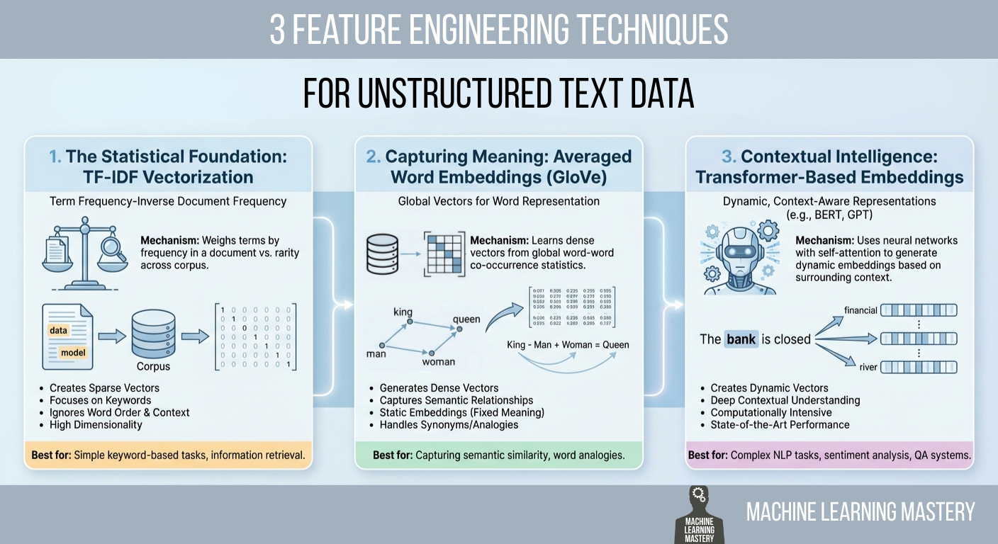
This text covers three distinct approaches to this drawback, starting from the statistical foundations of TF-IDF to the semantic averaging of GloVe vectors, and at last to the state-of-the-art contextual embeddings supplied by transformers.
1. The Statistical Basis: TF-IDF Vectorization
Essentially the most easy strategy to flip textual content into numbers is to rely them. This was the usual for many years. You’ll be able to merely rely the variety of instances a phrase seems in a doc, a way often known as bag of phrases. Nevertheless, uncooked counts have a major flaw. In virtually any English textual content, essentially the most frequent phrases are grammatically crucial however semantically empty articles and prepositions like “the,” “is,” “and,” or “of.” In case you depend on uncooked counts, these frequent phrases will dominate your information, drowning out the uncommon, particular phrases that really give the doc its which means.
To unravel this, we use time period frequency–inverse doc frequency (TF-IDF). This system weighs phrases not simply by how typically they seem in a particular doc, however by how uncommon they’re throughout your entire dataset. It’s a statistical balancing act designed to penalize frequent phrases and reward distinctive ones.
The primary half, time period frequency (TF), measures how ceaselessly a time period happens in a doc. The second half, inverse doc frequency (IDF), measures the significance of a time period. The IDF rating is calculated by taking the logarithm of the overall variety of paperwork divided by the variety of paperwork that comprise the precise time period.
If the phrase “information” seems in each single doc in your dataset, its IDF rating approaches zero, successfully cancelling it out. Conversely, if the phrase “hallucination” seems in just one doc, its IDF rating could be very excessive. Whenever you multiply TF by IDF, the result’s a function vector that highlights precisely what makes a particular doc distinctive in comparison with the others.
Implementation and Code Clarification
We are able to implement this effectively utilizing the scikit-learn TfidfVectorizer. On this instance, we take a small corpus of three sentences and convert them right into a matrix of numbers.
|
1 2 3 4 5 6 7 8 9 10 11 12 13 14 15 16 17 18 19 20 21 22 |
from sklearn.feature_extraction.textual content import TfidfVectorizer import pandas as pd
# 1. Outline a small corpus of textual content paperwork = [ “The quick brown fox jumps.”, “The quick brown fox runs fast.”, “The slow brown dog sleeps.” ]
# 2. Initialize the Vectorizer # We restrict the options to the highest 100 phrases to maintain the vector dimension manageable vectorizer = TfidfVectorizer(max_features=100)
# 3. Match and Rework the paperwork tfidf_matrix = vectorizer.fit_transform(paperwork)
# 4. View the end result as a DataFrame for readability feature_names = vectorizer.get_feature_names_out() df_tfidf = pd.DataFrame(tfidf_matrix.toarray(), columns=feature_names)
print(df_tfidf) |
The code begins by importing the mandatory TfidfVectorizer class. We outline a listing of strings that serves as our uncooked information. Once we name fit_transform, the vectorizer first learns the vocabulary of your entire checklist (the “match” step) after which transforms every doc right into a vector based mostly on that vocabulary.
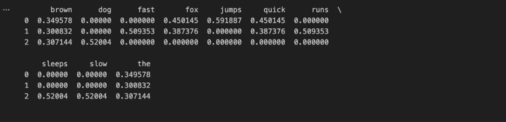
The output is a Pandas DataFrame, the place every row represents a sentence, and every column represents a novel phrase discovered within the information.
2. Capturing Which means: Averaged Phrase Embeddings (GloVe)
Whereas TF-IDF is highly effective for key phrase matching, it suffers from an absence of semantic understanding. It treats the phrases “good” and “wonderful” as utterly unrelated mathematical options as a result of they’ve completely different spellings. It doesn’t know that they imply practically the identical factor. To unravel this, we transfer to phrase embeddings.
Phrase embeddings are a way the place phrases are mapped to vectors of actual numbers. The core thought is that phrases with comparable meanings ought to have comparable mathematical representations. On this vector house, the space between the vector for “king” and “queen” is roughly just like the space between “man” and “girl.”
One of the crucial widespread pre-trained embedding units is GloVe (world vectors for phrase illustration), developed by researchers at Stanford. You’ll be able to entry their analysis and datasets on the official Stanford GloVe undertaking web page. These vectors have been educated on billions of phrases from Widespread Crawl and Wikipedia information. The mannequin seems to be at how typically phrases seem collectively (co-occurrence) to find out their semantic relationship.
To make use of this for function engineering, we face a small hurdle. GloVe supplies a vector for a single phrase, however our information normally consists of sentences or paragraphs. A standard, efficient method to symbolize a complete sentence is to calculate the imply of the vectors of the phrases it incorporates. You probably have a sentence with ten phrases, you lookup the vector for every phrase and common them collectively. The result’s a single vector that represents the “common which means” of your entire sentence.
Implementation and Code Clarification
For this instance, we are going to assume you will have downloaded a GloVe file (equivalent to glove.6B.50d.txt) from the Stanford hyperlink above. The code under hundreds these vectors into reminiscence and averages them for a pattern sentence.
|
1 2 3 4 5 6 7 8 9 10 11 12 13 14 15 16 17 18 19 20 21 22 23 24 25 26 27 28 29 30 31 32 33 34 35 36 37 38 39 40 41 42 43 44 |
import numpy as np
# 1. Load the GloVe embeddings right into a dictionary # This assumes you will have the glove.6B.50d.txt file domestically embeddings_index = {} with open(‘glove.6B.50d.txt’, encoding=‘utf-8’) as f: for line in f: values = line.break up() phrase = values[0] coefs = np.asarray(values[1:], dtype=‘float32’) embeddings_index[word] = coefs
print(f“Loaded {len(embeddings_index)} phrase vectors.”)
# 2. Outline a perform to vectorize a sentence def get_average_word2vec(tokens, vector_dict, generate_missing=False, okay=50): if len(tokens) < 1: return np.zeros(okay)
# Extract the vector for every phrase if it exists in our dictionary feature_vec = np.zeros((okay,), dtype=“float32”) rely = 0
for phrase in tokens: if phrase in vector_dict: feature_vec = np.add(feature_vec, vector_dict[word]) rely += 1
if rely == 0: return function_vec
# Divide the sum by the rely to get the typical feature_vec = np.divide(feature_vec, rely) return function_vec
# 3. Apply to a brand new sentence sentence = “synthetic intelligence is fascinating”
# Easy tokenization by splitting on house tokens = sentence.decrease().break up()
sentence_vector = get_average_word2vec(tokens, embeddings_index) print(f“The vector has a form of: {sentence_vector.form}”) print(sentence_vector[:5]) # Print first 5 numbers |
The code first builds a dictionary the place the keys are English phrases, and the values are the corresponding NumPy arrays representing their GloVe vectors. The perform get_average_word2vec iterates by way of the phrases in our enter sentence. It checks if the phrase exists in our GloVe dictionary; if it does, it provides that phrase’s vector to a working complete.
Lastly, it divides that complete sum by the variety of phrases discovered. This operation collapses the variable-length sentence right into a fixed-length vector (on this case, 50 dimensions). This numerical illustration captures the semantic subject of the sentence. A sentence about “canine” may have a mathematical common very near a sentence about “puppies,” even when they share no frequent phrases, which is a giant enchancment over TF-IDF.
3. Contextual Intelligence: Transformer-Primarily based Embeddings
The averaging technique described above represented a serious leap ahead, nevertheless it launched a brand new drawback: it ignores order and context. Whenever you common vectors, “The canine bit the person” and “The person bit the canine” lead to the very same vector as a result of they comprise the very same phrases. Moreover, the phrase “financial institution” has the identical static GloVe vector no matter whether or not you’re sitting on a “river financial institution” or visiting a “monetary financial institution.”
To unravel this, we use transformers, particularly fashions like BERT (Bidirectional Encoder Representations from Transformers). Transformers don’t learn textual content sequentially from left to proper; they learn your entire sequence without delay utilizing a mechanism referred to as “self-attention.” This permits the mannequin to grasp that the which means of a phrase is outlined by the phrases round it.
Once we use a transformer for function engineering, we’re not essentially coaching a mannequin from scratch. As an alternative, we use a pre-trained mannequin as a function extractor. We feed our textual content into the mannequin, and we extract the output from the ultimate hidden layer. Particularly, fashions like BERT prepend a particular token to each sentence referred to as the [CLS] (classification) token. The vector illustration of this particular token after passing by way of the layers is designed to carry the combination understanding of your entire sequence.
That is at present thought-about a gold customary for textual content illustration. You’ll be able to learn the seminal paper concerning this structure, “Consideration Is All You Want,” or discover the documentation for the Hugging Face Transformers library, which has made these fashions accessible to Python builders.
Implementation and Code Clarification
We’ll use the transformers library by Hugging Face and PyTorch to extract these options. Observe that this technique is computationally heavier than the earlier two.
|
1 2 3 4 5 6 7 8 9 10 11 12 13 14 15 16 17 18 19 20 21 22 23 24 25 |
from transformers import BertTokenizer, BertModel import torch
# 1. Initialize the Tokenizer and the Mannequin # We use ‘bert-base-uncased’, a smaller, environment friendly model of BERT tokenizer = BertTokenizer.from_pretrained(‘bert-base-uncased’) mannequin = BertModel.from_pretrained(‘bert-base-uncased’)
# 2. Preprocess the textual content textual content = “The financial institution of the river is muddy.” # return_tensors=”pt” tells it to return PyTorch tensors inputs = tokenizer(textual content, return_tensors=“pt”)
# 3. Go the enter by way of the mannequin # We use ‘no_grad()’ as a result of we’re solely extracting options, not coaching with torch.no_grad(): outputs = mannequin(**inputs)
# 4. Extract the options # ‘last_hidden_state’ incorporates vectors for all phrases # We normally need the [CLS] token, which is at index 0 cls_embedding = outputs.last_hidden_state[:, 0, :]
print(f“Vector form: {cls_embedding.form}”) print(cls_embedding[0][:5]) |
On this block, we first load the BertTokenizer and BertModel. The tokenizer breaks the textual content into items that the mannequin acknowledges. We then move these tokens into the mannequin. The torch.no_grad() context supervisor is used right here to inform PyTorch that we don’t must calculate gradients, which saves reminiscence and computation since we’re solely doing inference (extraction), not coaching.
The outputs variable incorporates the activations from the final layer of the neural community. We slice this tensor to get [:, 0, :]. This particular slice targets the primary token of the sequence, the [CLS] token talked about earlier. This single vector (normally 768 numbers lengthy for BERT Base) incorporates a deep, context-aware illustration of the sentence. Not like the GloVe common, this vector “is aware of” that the phrase “financial institution” on this sentence refers to a river as a result of it “paid consideration” to the phrases “river” and “muddy” throughout processing.
Conclusion
We’ve traversed the panorama of textual content function engineering from the straightforward to the delicate. We started with TF-IDF, a statistical technique that excels at key phrase matching and stays extremely efficient for easy doc retrieval or spam filtering. We moved to averaged phrase embeddings, equivalent to GloVe, which launched semantic which means and allowed fashions to grasp synonyms and analogies. Lastly, we examined transformer-based embeddings, which supply deep, context-aware representations that underpin essentially the most superior synthetic intelligence functions at present.
There isn’t a single “finest” method amongst these three; there’s solely the best method in your constraints. TF-IDF is quick, interpretable, and requires no heavy {hardware}. Transformers present the best accuracy however require vital computational energy and reminiscence. As an information scientist or engineer, your position is to strike a stability between these trade-offs to construct the simplest answer in your particular drawback.


