Massive Language Fashions (LLMs) can produce diverse, inventive, and generally shocking outputs even when given the identical immediate. This randomness is just not a bug however a core function of how the mannequin samples its subsequent token from a chance distribution. On this article, we break down the important thing sampling methods and display how parameters resembling temperature, top-okay, and top-p affect the stability between consistency and creativity.
On this tutorial, we take a hands-on strategy to grasp:
- How logits grow to be possibilities
- How temperature, top-okay, and top-p sampling work
- How completely different sampling methods form the mannequin’s next-token distribution
By the tip, you’ll perceive the mechanics behind LLM inference and be capable to alter the creativity or determinism of the output.
Let’s get began.

How LLMs Select Their Phrases: A Sensible Stroll-By means of of Logits, Softmax and Sampling
Photograph by Colton Duke. Some rights reserved.
Overview
This text is split into 4 components; they’re:
- How Logits Turn out to be Possibilities
- Temperature
- Prime-okay Sampling
- Prime-p Sampling
How Logits Turn out to be Possibilities
While you ask an LLM a query, it outputs a vector of logits. Logits are uncooked scores the mannequin assigns to every doable subsequent token in its vocabulary.
If the mannequin has a vocabulary of $V$ tokens, it should output a vector of $V$ logits for every subsequent phrase place. A logit is an actual quantity. It’s transformed right into a chance by the softmax perform:
$$
p_i = frac{e^{x_i}}{sum_{j=1}^{V} e^{x_j}}
$$
the place $x_i$ is the logit for token $i$ and $p_i$ is the corresponding chance. Softmax transforms these uncooked scores right into a chance distribution. All $p_i$ are constructive, and their sum is 1.
Suppose we give the mannequin this immediate:
At the moment’s climate is so ___
The mannequin considers each token in its vocabulary as a doable subsequent phrase. For simplicity, let’s say there are solely 6 tokens within the vocabulary:
|
great cloudy good scorching gloomy scrumptious |
The mannequin produces one logit for every token. Right here’s an instance set of logits the mannequin may output and the corresponding possibilities primarily based on the softmax perform:
| Token | Logit | Likelihood |
|---|---|---|
| great | 1.2 | 0.0457 |
| cloudy | 2.0 | 0.1017 |
| good | 3.5 | 0.4556 |
| scorching | 3.0 | 0.2764 |
| gloomy | 1.8 | 0.0832 |
| scrumptious | 1.0 | 0.0374 |
You’ll be able to verify this by utilizing the softmax perform from PyTorch:
|
import torch import torch.nn.purposeful as F
vocab = [“wonderful”, “cloudy”, “nice”, “hot”, “gloomy”, “delicious”] logits = torch.tensor([1.2, 2.0, 3.5, 3.0, 1.8, 1.0]) probs = F.softmax(logits, dim=–1) print(probs) # Output: # tensor([0.0457, 0.1017, 0.4556, 0.2764, 0.0832, 0.0374]) |
Based mostly on this end result, the token with the very best chance is “good”. LLMs don’t all the time choose the token with the very best chance; as a substitute, they pattern from the chance distribution to provide a distinct output every time. On this case, there’s a 46% chance of seeing “good”.
In order for you the mannequin to offer a extra inventive reply, how are you going to change the chance distribution such that “cloudy”, “scorching”, and different solutions would additionally seem extra typically?
Temperature
Temperature ($T$) is a mannequin inference parameter. It isn’t a mannequin parameter; it’s a parameter of the algorithm that generates the output. It scales logits earlier than making use of softmax:
$$
p_i = frac{e^{x_i / T}}{sum_{j=1}^{V} e^{x_j / T}}
$$
You’ll be able to anticipate the chance distribution to be extra deterministic if $T<1$, for the reason that distinction between every worth of $x_i$ might be exaggerated. However, it is going to be extra random if $T>1$, because the distinction between every worth of $x_i$ might be lowered.
Now, let’s visualize this impact of temperature on the chance distribution:
|
1 2 3 4 5 6 7 8 9 10 11 12 13 14 15 16 17 18 19 20 21 22 23 24 25 |
import matplotlib.pyplot as plt import torch import torch.nn.purposeful as F
vocab = [“wonderful”, “cloudy”, “nice”, “hot”, “gloomy”, “delicious”] logits = torch.tensor([1.2, 2.0, 3.5, 3.0, 1.8, 1.0]) # (vocab_size,) scores = logits.unsqueeze(0) # (1, vocab_size) temperatures = [0.1, 0.5, 1.0, 3.0, 10.0]
fig, ax = plt.subplots(figsize=(10, 6)) for temp in temperatures: # Apply temperature scaling scores_processed = scores / temp # Convert to possibilities probs = F.softmax(scores_processed, dim=–1)[0] # Pattern from the distribution sampled_idx = torch.multinomial(probs, num_samples=1).merchandise() print(f“Temperature = {temp}, sampled: {vocab[sampled_idx]}”) # Plot the chance distribution ax.plot(vocab, probs.numpy(), marker=‘o’, label=f“T={temp}”)
ax.set_title(“Impact of Temperature”) ax.set_ylabel(“Likelihood”) ax.legend() plt.present() |
This code generates a chance distribution over every token within the vocabulary. Then it samples a token primarily based on the chance. Operating this code could produce the next output:
|
Temperature = 0.1, sampled: good Temperature = 0.5, sampled: good Temperature = 1.0, sampled: good Temperature = 3.0, sampled: great Temperature = 10.0, sampled: scrumptious |
and the next plot exhibiting the chance distribution for every temperature:
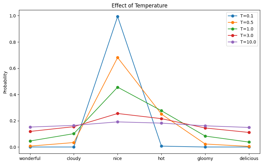
The impact of temperature to the ensuing chance distribution
The mannequin could produce the nonsensical output “At the moment’s climate is so scrumptious” when you set the temperature to 10!
Prime-okay Sampling
The mannequin’s output is a vector of logits for every place within the output sequence. The inference algorithm converts the logits to precise phrases, or in LLM phrases, tokens.
The only technique for choosing the subsequent token is grasping sampling, which all the time selects the token with the very best chance. Whereas environment friendly, this typically yields repetitive, predictable output. One other technique is to pattern the token from the softmax-probability distribution derived from the logits. Nevertheless, as a result of an LLM has a really giant vocabulary, inference is gradual, and there’s a small likelihood of manufacturing nonsensical tokens.
Prime-$okay$ sampling strikes a stability between determinism and creativity. As an alternative of sampling from your complete vocabulary, it restricts the candidate pool to the highest $okay$ most possible tokens and samples from that subset. Tokens exterior this top-$okay$ group are assigned zero chance and can by no means be chosen. It not solely accelerates inference by lowering the efficient vocabulary measurement, but in addition eliminates tokens that shouldn’t be chosen.
By filtering out extraordinarily unlikely tokens whereas nonetheless permitting randomness among the many most believable ones, top-$okay$ sampling helps keep coherence with out sacrificing variety. When $okay=1$, top-$okay$ reduces to grasping sampling.
Right here is an instance of how one can implement top-$okay$ sampling:
|
1 2 3 4 5 6 7 8 9 10 11 12 13 14 15 16 17 18 19 20 21 22 23 24 25 26 27 28 29 30 |
import matplotlib.pyplot as plt import torch import torch.nn.purposeful as F
vocab = [“wonderful”, “cloudy”, “nice”, “hot”, “gloomy”, “delicious”] logits = torch.tensor([1.2, 2.0, 3.5, 3.0, 1.8, 1.0]) # (vocab_size,) scores = logits.unsqueeze(0) # (batch, vocab_size) k_candidates = [1, 2, 3, 6]
fig, ax = plt.subplots(figsize=(10, 6)) for top_k in k_candidates: # 1. get the top-k logits topk_values = torch.topk(scores, top_k)[0] # 2. threshold = smallest logit contained in the top-k set threshold = topk_values[..., –1, None] # (…, 1) # 3. masks all logits beneath the edge to -inf indices_to_remove = scores < threshold filtered_scores = scores.masked_fill(indices_to_remove, –float(“inf”)) # convert to possibilities, these with -inf logits will get zero chance probs = F.softmax(filtered_scores, dim=–1)[0] # pattern from the filtered distribution sampled_idx = torch.multinomial(probs, num_samples=1).merchandise() print(f“Prime-k = {top_k}, sampled: {vocab[sampled_idx]}”) # Plot the chance distribution ax.plot(vocab, probs.numpy(), marker=‘o’, label=f“Prime-k = {top_k}”)
ax.set_title(“Impact of Prime-k Sampling”) ax.set_ylabel(“Likelihood”) ax.legend() plt.present() |
This code modifies the earlier instance by filling some tokens’ logits with $-infty$ to make the chance of these tokens zero. Operating this code could produce the next output:
|
Prime-k = 1, sampled: good Prime-k = 2, sampled: good Prime-k = 3, sampled: scorching Prime-k = 6, sampled: scrumptious |
The next plot reveals the chance distribution after top-$okay$ filtering:
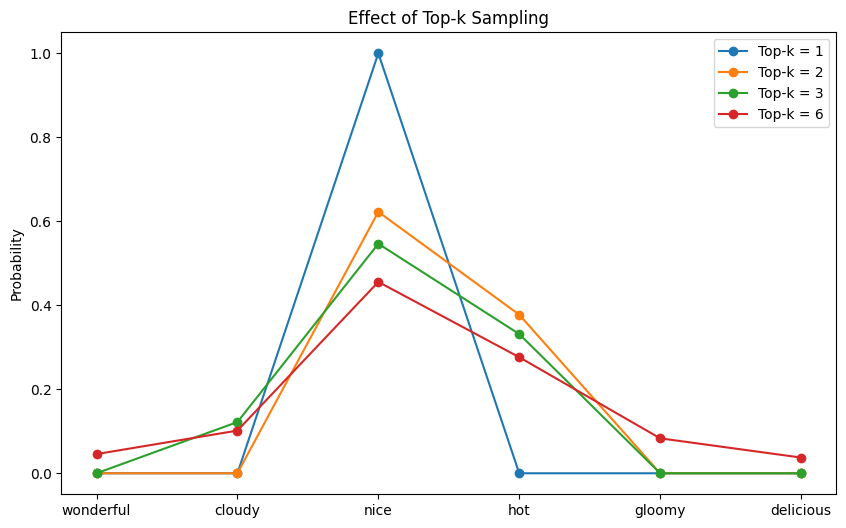
The chance distribution after top-$okay$ filtering
You’ll be able to see that for every $okay$, the chances of precisely $V-k$ tokens are zero. These tokens won’t ever be chosen beneath the corresponding top-$okay$ setting.
Prime-p Sampling
The issue with top-$okay$ sampling is that it all the time selects from a set variety of tokens, no matter how a lot chance mass they collectively account for. Sampling from even the highest $okay$ tokens can nonetheless enable the mannequin to select from the lengthy tail of low-probability choices, which regularly results in incoherent output.
Prime-$p$ sampling (often known as nucleus sampling) addresses this concern by sampling tokens in line with their cumulative chance somewhat than a set rely. It selects the smallest set of tokens whose cumulative chance exceeds a threshold $p$, successfully making a dynamic $okay$ for every place to filter out unreliable tail possibilities whereas retaining solely probably the most believable candidates. When the mannequin is sharp and peaked, top-$p$ yields fewer candidate tokens; when the distribution is flat, it expands accordingly.
Setting $p$ near 1.0 approaches full sampling from all tokens. Setting $p$ to a really small worth makes the sampling extra conservative. Right here is how one can implement top-$p$ sampling:
|
1 2 3 4 5 6 7 8 9 10 11 12 13 14 15 16 17 18 19 20 21 22 23 24 25 26 27 28 29 30 31 32 33 34 35 36 |
import matplotlib.pyplot as plt import torch import torch.nn.purposeful as F
vocab = [“wonderful”, “cloudy”, “nice”, “hot”, “gloomy”, “delicious”] logits = torch.tensor([1.2, 2.0, 3.5, 3.0, 1.8, 1.0]) # (vocab_size,) scores = logits.unsqueeze(0) # (1, vocab_size)
p_candidates = [0.3, 0.6, 0.8, 0.95, 1.0] fig, ax = plt.subplots(figsize=(10, 6)) for top_p in p_candidates: # 1. type logits in ascending order sorted_logits, sorted_indices = torch.type(scores, descending=False) # 2. compute possibilities of the sorted logits sorted_probs = F.softmax(sorted_logits, dim=–1) # 3. cumulative probs from low-prob tokens to high-prob tokens cumulative_probs = sorted_probs.cumsum(dim=–1) # 4. take away tokens with cumulative top_p above the edge (token with 0 are saved) sorted_indices_to_remove = cumulative_probs <= (1.0 – top_p) # 5. preserve not less than 1 token, which is the one with highest chance sorted_indices_to_remove[..., –1:] = 0 # 6. scatter sorted tensors to unique indexing indices_to_remove = sorted_indices_to_remove.scatter(1, sorted_indices, sorted_indices_to_remove) # 7. masks logits of tokens to take away with -inf scores_processed = scores.masked_fill(indices_to_remove, –float(“inf”)) # possibilities after top-p filtering, these with -inf logits will get zero chance probs = F.softmax(scores_processed, dim=–1)[0] # (vocab_size,) # pattern from nucleus distribution choice_idx = torch.multinomial(probs, num_samples=1).merchandise() print(f“Prime-p = {top_p}, sampled: {vocab[choice_idx]}”) ax.plot(vocab, probs.numpy(), marker=‘o’, label=f“Prime-p = {top_p}”)
ax.set_title(“Impact of Prime-p (Nucleus) Sampling”) ax.set_ylabel(“Likelihood”) ax.legend() plt.present() |
Operating this code could produce the next output:
|
Prime-p = 0.3, sampled: good Prime-p = 0.6, sampled: scorching Prime-p = 0.8, sampled: good Prime-p = 0.95, sampled: scorching Prime-p = 1.0, sampled: scorching |
and the next plot reveals the chance distribution after top-$p$ filtering:
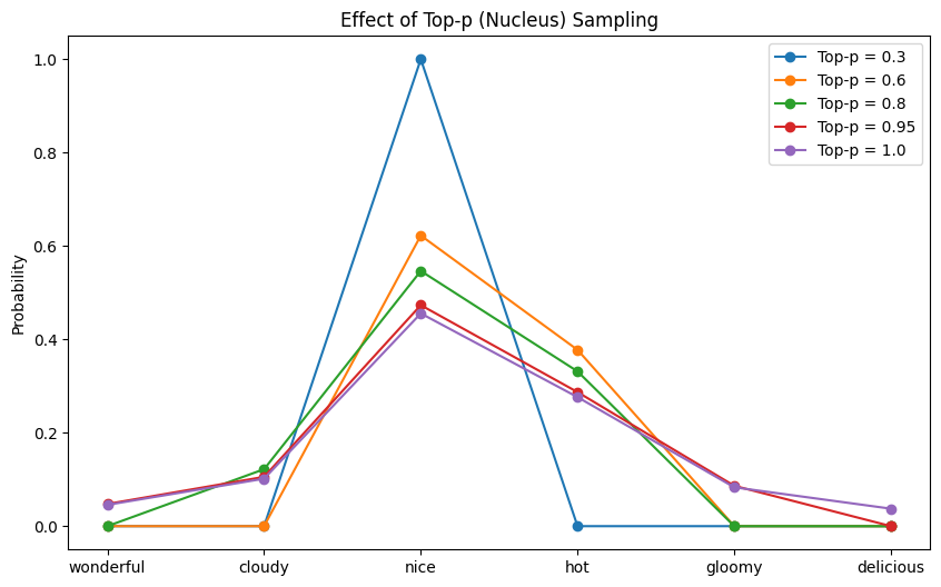
The chance distribution after top-$p$ filtering
From this plot, you might be much less more likely to see the impact of $p$ on the variety of tokens with zero chance. That is the supposed conduct because it depends upon the mannequin’s confidence within the subsequent token.
Additional Readings
Under are some additional readings that you could be discover helpful:
Abstract
This text demonstrated how completely different sampling methods have an effect on an LLM’s selection of subsequent phrase in the course of the decoding part. You realized to pick out completely different values for the temperature, top-$okay$, and top-$p$ sampling parameters for various LLM use circumstances.


