Transformer vs LSTM for Time Collection: Which Works Higher?

On this article, you’ll learn to construct, prepare, and examine an LSTM and a transformer for next-day univariate time collection forecasting on actual public transit information.

Subjects we are going to cowl embody:

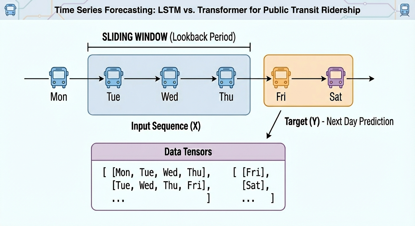
Structuring and windowing a time collection for supervised studying.
Implementing compact LSTM and transformer architectures in PyTorch.
Evaluating and evaluating fashions with MAE and RMSE on held-out information.

All proper, full steam forward.

Transformer vs LSTM for Time Series: Which Works Better?

Transformer vs LSTM for Time Collection: Which Works Higher?
Picture by Editor

Introduction

From day by day climate measurements or site visitors sensor readings to inventory costs, time collection information are current almost all over the place. When these time collection datasets change into tougher, fashions with a better stage of sophistication — resembling ensemble strategies and even deep studying architectures — is usually a extra handy possibility than classical time collection evaluation and forecasting strategies.

The target of this text is to showcase how two deep studying architectures are educated and used to deal with time collection information — lengthy quick time period reminiscence (LSTM) and the transformer. The primary focus just isn’t merely leveraging the fashions, however understanding their variations when dealing with time collection and whether or not one structure clearly outperforms the opposite. Primary information of Python and machine studying necessities is advisable.

Downside Setup and Preparation

For this illustrative comparability, we are going to contemplate a forecasting activity on a univariate time collection: given the temporally ordered earlier N time steps, predict the (N+1)th worth.

Specifically, we are going to use a publicly accessible model of the Chicago rides dataset, which incorporates day by day recordings for bus and rail passengers within the Chicago public transit community courting again to 2001.

This preliminary piece of code imports the libraries and modules wanted and masses the dataset. We’ll import pandas, NumPy, Matplotlib, and PyTorch — all for the heavy lifting — together with the scikit-learn metrics that we are going to depend on for analysis.

import pandas as pd import numpy as np import matplotlib.pyplot as plt import torch import torch.nn as nn from sklearn.metrics import mean_squared_error, mean_absolute_error url = “https://information.cityofchicago.org/api/views/6iiy-9s97/rows.csv?accessType=DOWNLOAD” df = pd.read_csv(url, parse_dates=[“service_date”]) print(df.head())

import pandas as pd

import numpy as np

import matplotlib.pyplot as plt

import torch

import torch.nn as nn

from sklearn.metrics import mean_squared_error, mean_absolute_error

url = “https://information.cityofchicago.org/api/views/6iiy-9s97/rows.csv?accessType=DOWNLOAD”

df = pd.read_csv(url, parse_dates=[“service_date”])

print(df.head())

For the reason that dataset incorporates post-COVID actual information about passenger numbers — which can severely mislead the predictive energy of our fashions as a result of being very in another way distributed than pre-COVID information — we are going to filter out information from January 1, 2020 onwards.

df_filtered = df[df[‘service_date’] <= ‘2019-12-31’] print(“Filtered DataFrame head:”) show(df_filtered.head()) print(“nShape of the filtered DataFrame:”, df_filtered.form) df = df_filtered

df_filtered = df[df[‘service_date’] <= ‘2019-12-31’]

print(“Filtered DataFrame head:”)

show(df_filtered.head())

print(“nShape of the filtered DataFrame:”, df_filtered.form)

df = df_filtered

A easy plot will do the job to indicate what the filtered information seems like:

df.sort_values(“service_date”, inplace=True) ts = df.set_index(“service_date”)[“total_rides”].fillna(0) plt.plot(ts) plt.title(“CTA Day by day Complete Rides”) plt.present()

df.sort_values(“service_date”, inplace=True)

ts = df.set_index(“service_date”)[“total_rides”].fillna(0)

plt.plot(ts)

plt.title(“CTA Day by day Complete Rides”)

plt.present()

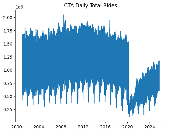
Chicago rides time collection dataset plotted

Subsequent, we cut up the time collection information into coaching and take a look at units. Importantly, in time collection forecasting duties — not like classification and regression — this partition can’t be finished at random, however in a purely sequential vogue. In different phrases, all coaching situations come chronologically first, adopted by take a look at situations. This code takes the primary 80% of the time collection as a coaching set, and the remaining 20% for testing.

n = len(ts) prepare = ts[:int(0.8*n)] take a look at = ts[int(0.8*n):] train_vals = prepare.values.astype(float) test_vals = take a look at.values.astype(float)

n = len(ts)

prepare = ts[:int(0.8*n)]

take a look at = ts[int(0.8*n):]

train_vals = prepare.values.astype(float)

test_vals = take a look at.values.astype(float)

Moreover, uncooked time collection have to be transformed into labeled sequences (x, y) spanning a set time window to correctly prepare neural network-based fashions upon them. For instance, if we use a time window of N=30 days, the primary occasion will span the primary 30 days of the time collection, and the related label to foretell would be the thirty first day, and so forth. This offers the dataset an acceptable labeled format for supervised studying duties with out dropping its necessary temporal which means:

def create_sequences(information, seq_len=30): X, y = [], [] for i in vary(len(information)-seq_len): X.append(information[i:i+seq_len]) y.append(information[i+seq_len]) return np.array(X), np.array(y) SEQ_LEN = 30 X_train, y_train = create_sequences(train_vals, SEQ_LEN) X_test, y_test = create_sequences(test_vals, SEQ_LEN) # Convert our formatted information into PyTorch tensors X_train = torch.tensor(X_train).float().unsqueeze(-1) y_train = torch.tensor(y_train).float().unsqueeze(-1) X_test = torch.tensor(X_test).float().unsqueeze(-1) y_test = torch.tensor(y_test).float().unsqueeze(-1)

def create_sequences(information, seq_len=30):

X, y = [], []

for i in vary(len(information)–seq_len):

X.append(information[i:i+seq_len])

y.append(information[i+seq_len])

return np.array(X), np.array(y)

SEQ_LEN = 30

X_train, y_train = create_sequences(train_vals, SEQ_LEN)

X_test, y_test = create_sequences(test_vals, SEQ_LEN)

# Convert our formatted information into PyTorch tensors

X_train = torch.tensor(X_train).float().unsqueeze(–1)

y_train = torch.tensor(y_train).float().unsqueeze(–1)

X_test = torch.tensor(X_test).float().unsqueeze(–1)

y_test = torch.tensor(y_test).float().unsqueeze(–1)

We at the moment are prepared to coach, consider, and examine our LSTM and transformer fashions!

Mannequin Coaching

We’ll use the PyTorch library for the modeling stage, because it supplies the mandatory lessons to outline each recurrent LSTM layers and encoder-only transformer layers appropriate for predictive duties.

First up, we’ve an LSTM-based RNN structure like this:

class LSTMModel(nn.Module): def __init__(self, hidden=32): tremendous().__init__() self.lstm = nn.LSTM(1, hidden, batch_first=True) self.fc = nn.Linear(hidden, 1) def ahead(self, x): out, _ = self.lstm(x) return self.fc(out[:, -1]) lstm_model = LSTMModel()

class LSTMModel(nn.Module):

def __init__(self, hidden=32):

tremendous().__init__()

self.lstm = nn.LSTM(1, hidden, batch_first=True)

self.fc = nn.Linear(hidden, 1)

def ahead(self, x):

out, _ = self.lstm(x)

return self.fc(out[:, –1])

lstm_model = LSTMModel()

As for the encoder-only transformer for next-day time collection forecasting, we’ve:

class SimpleTransformer(nn.Module): def __init__(self, d_model=32, nhead=4): tremendous().__init__() self.embed = nn.Linear(1, d_model) enc_layer = nn.TransformerEncoderLayer(d_model=d_model, nhead=nhead, batch_first=True) self.transformer = nn.TransformerEncoder(enc_layer, num_layers=1) self.fc = nn.Linear(d_model, 1) def ahead(self, x): x = self.embed(x) x = self.transformer(x) return self.fc(x[:, -1]) transformer_model = SimpleTransformer()

class SimpleTransformer(nn.Module):

def __init__(self, d_model=32, nhead=4):

tremendous().__init__()

self.embed = nn.Linear(1, d_model)

enc_layer = nn.TransformerEncoderLayer(d_model=d_model, nhead=nhead, batch_first=True)

self.transformer = nn.TransformerEncoder(enc_layer, num_layers=1)

self.fc = nn.Linear(d_model, 1)

def ahead(self, x):

x = self.embed(x)

x = self.transformer(x)

return self.fc(x[:, –1])

transformer_model = SimpleTransformer()

Notice that the final layer in each architectures follows an identical sample: its enter form is the hidden illustration dimensionality (32 in our instance), and one single neuron is used to carry out a single forecast of the next-day complete rides.

Time to coach the fashions and consider each fashions’ efficiency with the take a look at information:

def prepare(mannequin, X, y, epochs=10): mannequin.prepare() choose = torch.optim.Adam(mannequin.parameters(), lr=1e-3) loss_fn = nn.MSELoss() for epoch in vary(epochs): choose.zero_grad() out = mannequin(X) loss = loss_fn(out, y) loss.backward() choose.step() return mannequin lstm_model = prepare(lstm_model, X_train, y_train) transformer_model = prepare(transformer_model, X_train, y_train)

def prepare(mannequin, X, y, epochs=10):

mannequin.prepare()

choose = torch.optim.Adam(mannequin.parameters(), lr=1e–3)

loss_fn = nn.MSELoss()

for epoch in vary(epochs):

choose.zero_grad()

out = mannequin(X)

loss = loss_fn(out, y)

loss.backward()

choose.step()

return mannequin

lstm_model = prepare(lstm_model, X_train, y_train)

transformer_model = prepare(transformer_model, X_train, y_train)

We’ll examine how the fashions carried out for a univariate time collection forecasting activity utilizing two frequent metrics: imply absolute error (MAE) and root imply squared error (RMSE).

lstm_model.eval() transformer_model.eval() pred_lstm = lstm_model(X_test).detach().numpy().flatten() pred_trans = transformer_model(X_test).detach().numpy().flatten() true_vals = y_test.numpy().flatten() rmse_lstm = np.sqrt(mean_squared_error(true_vals, pred_lstm)) mae_lstm = mean_absolute_error(true_vals, pred_lstm) rmse_trans = np.sqrt(mean_squared_error(true_vals, pred_trans)) mae_trans = mean_absolute_error(true_vals, pred_trans) print(f”LSTM RMSE={rmse_lstm:.1f}, MAE={mae_lstm:.1f}”) print(f”Trans RMSE={rmse_trans:.1f}, MAE={mae_trans:.1f}”)

lstm_model.eval()

transformer_model.eval()

pred_lstm = lstm_model(X_test).detach().numpy().flatten()

pred_trans = transformer_model(X_test).detach().numpy().flatten()

true_vals = y_test.numpy().flatten()

rmse_lstm = np.sqrt(mean_squared_error(true_vals, pred_lstm))

mae_lstm = mean_absolute_error(true_vals, pred_lstm)

rmse_trans = np.sqrt(mean_squared_error(true_vals, pred_trans))

mae_trans = mean_absolute_error(true_vals, pred_trans)

print(f“LSTM RMSE={rmse_lstm:.1f}, MAE={mae_lstm:.1f}”)

print(f“Trans RMSE={rmse_trans:.1f}, MAE={mae_trans:.1f}”)

Outcomes Dialogue

Listed here are the outcomes we obtained:

LSTM RMSE=1350000.8, MAE=1297517.9 Trans RMSE=1349997.3, MAE=1297514.1

LSTM RMSE=1350000.8, MAE=1297517.9

Trans RMSE=1349997.3, MAE=1297514.1

The outcomes are extremely comparable between the 2 fashions, making it tough to find out whether or not one is best than the opposite (if we glance carefully, the transformer performs a tiny bit higher, however the distinction is actually negligible).

Why are the outcomes so comparable? Univariate time collection forecasting on information that observe a fairly constant sample over time, such because the dataset we contemplate, can yield comparable outcomes throughout these fashions as a result of each have sufficient capability to resolve this downside — regardless that the complexity of every structure right here is deliberately minimal. I counsel you strive your complete course of once more with out filtering the post-COVID situations, maintaining the identical 80/20 ratio for coaching and testing over your complete authentic dataset, and see if the distinction between the 2 fashions will increase (be at liberty to remark under together with your findings).

In addition to, the forecasting activity may be very short-term: we’re simply predicting the next-day worth, as a substitute of getting a extra complicated label set y that spans a subsequent time window to the one thought-about for inputs X. If we predicted values 30 days forward, the distinction between the fashions’ errors would doubtless widen, with the transformer arguably outperforming the LSTM (though this won’t at all times be the case).

Wrapping Up

This text showcased the best way to handle a time collection forecasting activity with two totally different deep studying architectures: LSTM and the transformer. We guided you thru your complete course of, from acquiring the information to coaching the fashions, evaluating them, evaluating, and deciphering outcomes.