Create Interactive, Droplet-like Metaballs with Three.js and GLSL

Fragment shaders permit us to create clean, natural visuals which are tough to attain with customary polygon-based rendering in WebGL. One highly effective instance is the metaball impact, the place a number of objects mix and deform seamlessly. This may be carried out utilizing a way referred to as ray marching, immediately inside a fraction shader.

On this tutorial, we’ll stroll you thru the way to create droplet-like, bubble spheres utilizing Three.js and GLSL—an impact that responds interactively to your mouse actions. However first, check out the demo video beneath to see the ultimate end in motion.

Overview

Let’s check out the general construction of the demo and evaluate the steps we’ll comply with to construct it.

1. Setting Up the Fullscreen Airplane

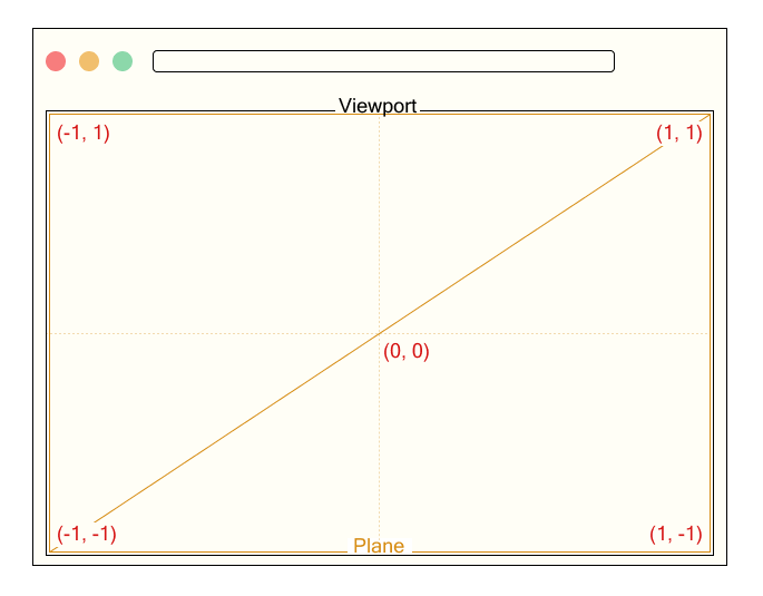
We create a fullscreen aircraft that covers the complete viewport.

2. Rendering Spheres with Ray Marching

We’ll render spheres utilizing ray marching within the fragment shader.

3. From Spheres to Metaballs

We mix a number of spheres easily to create a metaball impact.

4. Including Noise for a Droplet-like Look

By including noise to the floor, we create a sensible droplet-like texture.

5. Simulating Stretchy Droplets with Mouse Motion

We prepare spheres alongside the mouse path to create a stretchy, elastic movement.

Let’s get began!

1. Setup

We render a single fullscreen aircraft that covers the complete viewport.

// Output.ts

const planeGeometry = new THREE.PlaneGeometry(2.0, 2.0);
const planeMaterial = new THREE.RawShaderMaterial({
    vertexShader: base_vert,
    fragmentShader: output_frag,
    uniforms: this.uniforms,
});
const aircraft = new THREE.Mesh(planeGeometry, planeMaterial);
this.scene.add(aircraft);

We outline a uniform variable named uResolution to move the canvas dimension to the shader, the place Widespread.width and Widespread.top characterize the width and top of the canvas in pixels. This uniform shall be used to normalize coordinates primarily based on the display decision.

// Output.ts

this.uniforms = {
    uResolution: {
        worth: new THREE.Vector2(Widespread.width, Widespread.top),
    },
};

When utilizing RawShaderMaterial, it’s essential present your personal shaders. Due to this fact, we put together each a vertex shader and a fraction shader.

// base.vert

attribute vec3 place;
various vec2 vTexCoord;

void predominant() {
    vTexCoord = place.xy * 0.5 + 0.5;
    gl_Position = vec4(place, 1.0);
}

The vertex shader receives the place attribute.

Because the xy elements of place initially vary from -1 to 1, we convert them to a spread from 0 to 1 and output them as a texture coordinate referred to as vTexCoord. That is handed to the fragment shader and used to calculate colours or results primarily based on the place on the display.

// output.frag

precision mediump float;

uniform vec2 uResolution;
various vec2 vTexCoord;

void predominant() {
    gl_FragColor = vec4(vTexCoord, 1.0, 1.0);
}

The fragment shader receives the interpolated texture coordinate vTexCoord and the uniform variable uResolution representing the canvas dimension. Right here, we briefly use vTexCoord to output coloration for testing.

Now we’re all set to begin drawing within the fragment shader!
Subsequent, let’s transfer on to really rendering the spheres.

2. Ray Marching

2.1. What’s Ray Marching?

As talked about at the start, we’ll use a way referred to as ray marching to render spheres. Ray marching proceeds within the following steps:

Outline the scene
Set the digicam (viewing) route
Forged rays
Consider the space from the present ray place to the closest object within the scene.
Transfer the ray ahead by that distance
Test for successful

For instance, let’s think about a scene with three spheres. These spheres are expressed utilizing SDFs (Signed Distance Capabilities), which shall be defined intimately later.

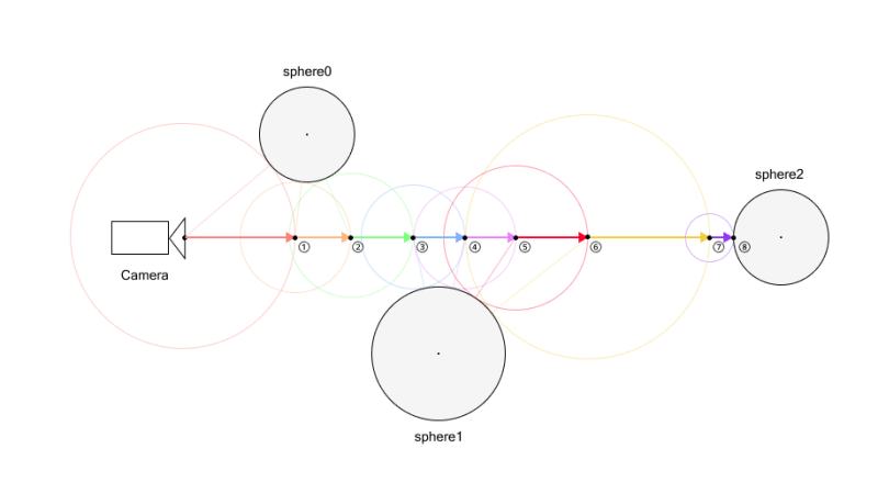
First, we decide the digicam route. As soon as the route is ready, we solid a ray in that route.

Subsequent, we consider the space to all objects from the present ray place, and take the minimal of those distances.

After acquiring this distance, we transfer the ray ahead by that quantity.

We repeat this course of till both the ray will get shut sufficient to an object—nearer than a small threshold—or the utmost variety of steps is reached.
If the space is beneath the brink, we think about it a “hit” and shade the corresponding pixel.

For instance, within the determine above, successful is detected on the eighth ray marching step.

If the utmost variety of steps had been set to 7, the seventh step wouldn’t have hit something but. However because the restrict is reached, the loop ends and no hit is detected.

Due to this fact, nothing could be rendered at that place. If components of an object seem like lacking within the ultimate picture, it could be resulting from an inadequate variety of steps. Nevertheless, remember that growing the step rely may also enhance the computational load.

To higher perceive this course of, strive working this demo to see the way it works in follow.

2.2. Signed Distance Operate

Within the earlier part, we briefly talked about the SDF (Signed Distance Operate).
Let’s take a second to know what it’s.

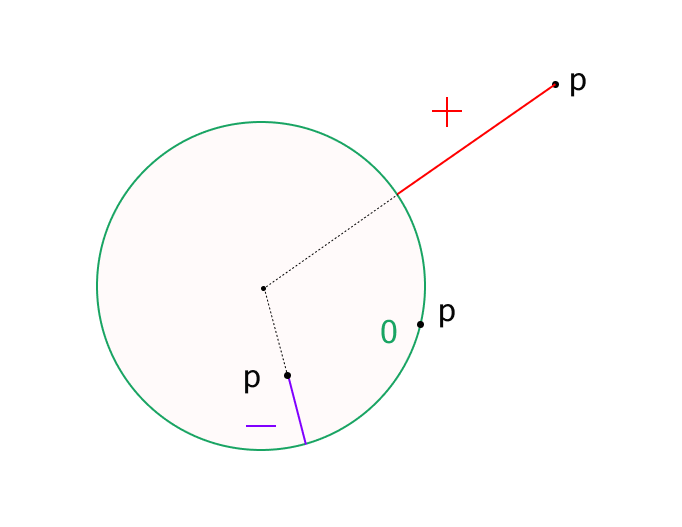
An SDF is a perform that returns the space from a degree to a specific form. The important thing attribute is that it returns a optimistic or unfavourable worth relying on whether or not the purpose is exterior or inside the form.

For instance, right here is the space perform for a sphere:

float sdSphere(vec3 p, float s)
{
    return size(p) - s;
}

Right here, p is a vector representing the place relative to the origin, and s is the radius of the sphere.

This perform calculates how far the purpose p is from the floor of a sphere centered on the origin with radius s.

If the result’s optimistic, the purpose is exterior the sphere.
If unfavourable, it’s inside the sphere.
If the result’s zero, the purpose is on the floor—that is thought of successful level (in follow, we detect successful when the space is lower than a small threshold).

On this demo, we use a sphere’s distance perform, however many different shapes have their very own distance features as nicely.

In the event you’re , right here’s an amazing article on distance features.

2.3. Rendering Spheres

Let’s strive rendering spheres.
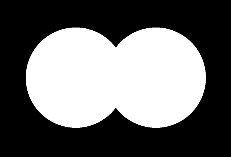
On this demo, we’ll render two barely overlapping spheres.

// output.frag

precision mediump float;

const float EPS = 1e-4;
const int ITR = 16;

uniform vec2 uResolution;

various vec2 vTexCoord;

// Digicam Params
vec3 origin = vec3(0.0, 0.0, 1.0);
vec3 lookAt = vec3(0.0, 0.0, 0.0);
vec3 cDir = normalize(lookAt - origin);
vec3 cUp = vec3(0.0, 1.0, 0.0);
vec3 cSide = cross(cDir, cUp);

vec3 translate(vec3 p, vec3 t) {
    return p - t;
}

float sdSphere(vec3 p, float s)
{
    return size(p) - s;
}

float map(vec3 p) {
    float radius = 0.5;
    float d = 1e5;

    float sphere0 = sdSphere(translate(p, vec3(0.4, 0.0, 0.0)), radius);
    float sphere1 = sdSphere(translate(p, vec3(-0.4, 0.0, 0.0)), radius);
    d = min(sphere0, sphere1);

    return d;
}

void predominant() {
    vec2 p = (gl_FragCoord.xy * 2.0 - uResolution) / min(uResolution.x, uResolution.y);

    // Orthographic Digicam
    vec3 ray = origin + cSide * p.x + cUp * p.y;
    vec3 rayDirection = cDir;

    float dist = 0.0;

    for (int i = 0; i < ITR; ++i) {
        dist = map(ray);
        ray += rayDirection * dist;
        if (dist < EPS) break;
    }

    vec3 coloration = vec3(0.0);

    if (dist < EPS) {
        coloration = vec3(1.0, 1.0, 1.0);
    }

    gl_FragColor = vec4(coloration, 1.0);
}

First, we normalize the display coordinates:

vec2 p = (gl_FragCoord.xy * 2.0 - uResolution) / min(uResolution.x, uResolution.y);

Subsequent, we arrange the digicam. This demo makes use of an orthographic digicam (parallel projection):

// Digicam Params
vec3 origin = vec3(0.0, 0.0, 1.0);
vec3 lookAt = vec3(0.0, 0.0, 0.0);
vec3 cDir = normalize(lookAt - origin);
vec3 cUp = vec3(0.0, 1.0, 0.0);
vec3 cSide = cross(cDir, cUp);

// Orthographic Digicam
vec3 ray = origin + cSide * p.x + cUp * p.y;
vec3 rayDirection = cDir;

After that, contained in the map perform, two spheres are outlined and their distances calculated utilizing sdSphere. The variable d is initially set to a big worth and up to date with the min perform to maintain observe of the shortest distance to the floor.

float map(vec3 p) {
    float radius = 0.5;
    float d = 1e5;

    float sphere0 = sdSphere(translate(p, vec3(0.4, 0.0, 0.0)), radius);
    float sphere1 = sdSphere(translate(p, vec3(-0.4, 0.0, 0.0)), radius);
    d = min(sphere0, sphere1);

    return d;
}

Then we run a ray marching loop, which updates the ray place by computing the space to the closest object at every step. The loop ends both after a hard and fast variety of iterations or when the space turns into smaller than a threshold (dist < EPS):

for ( int i = 0; i < ITR; ++ i ) {
	dist = map(ray);
	ray += rayDirection * dist;
	if ( dist < EPS ) break ;
}

Lastly, we decide the output coloration. We use black because the default coloration (background), and render a white pixel provided that successful is detected:

vec3 coloration = vec3(0.0);

if ( dist < EPS ) {
	coloration = vec3(1.0);
}

We’ve efficiently rendered two overlapping spheres utilizing ray marching!

2.4. Normals

Though we efficiently rendered spheres within the earlier part, the scene nonetheless seems flat and lacks depth. It is because we haven’t utilized any shading or visible results that reply to floor orientation.

Whereas we received’t implement full shading on this demo, we’ll nonetheless compute floor normals, as they’re important for including floor element and different visible results.

Let’s take a look at the code first:

vec3 generateNormal(vec3 p) {
    return normalize(vec3(
            map(p + vec3(EPS, 0.0, 0.0)) - map(p + vec3(-EPS, 0.0, 0.0)),
            map(p + vec3(0.0, EPS, 0.0)) - map(p + vec3(0.0, -EPS, 0.0)),
            map(p + vec3(0.0, 0.0, EPS)) - map(p + vec3(0.0, 0.0, -EPS))
        ));
}

At first look, this will appear onerous to know. Put merely, this computes the gradient of the space perform, which corresponds to the conventional vector.

In the event you’ve studied vector calculus, this may be simple to know. For a lot of others, although, it could appear a bit tough.

That’s completely effective—a full understanding of the small print isn’t essential to make use of the end result. In the event you simply need to transfer on, be at liberty to skip forward to the part the place we debug normals by visualizing them with coloration.

Nevertheless, for many who are occupied with the way it works, we’ll now stroll by way of the reason in additional element.

The gradient of a scalar perform 𝑓(𝑥,𝑦,𝑧) is just a vector composed of its partial derivatives. It factors within the route of the best charge of enhance of the perform:

To compute this gradient numerically, we will use the central distinction technique. For instance:

We apply the identical concept for the 𝑦 and 𝑧 elements.
Notice: The issue 2𝜀 is omitted within the code since we normalize the end result utilizing normalize().

Subsequent, allow us to think about a signed distance perform 𝑓(𝑥,𝑦,𝑧), which returns the shortest distance from any level in house to the floor of an object. By definition, 𝑓(𝑥,𝑦,𝑧)=0 on the floor of the item.

Assume that 𝑓 is clean (i.e., differentiable) within the area of curiosity. When the purpose (𝑥,𝑦,𝑧) undergoes a small displacement Δ𝒓=(Δ𝑥,Δ𝑦,Δ𝑧), the change within the perform worth Δ𝑓 could be approximated utilizing the first-order Taylor enlargement:

Right here,∇𝑓 is the gradient vector of 𝑓, and Δ𝒓 is an arbitrary small displacement vector.

Now, since 𝑓=0 on the floor and stays fixed as we transfer alongside the floor (i.e., tangentially), the perform worth doesn’t change, so Δ𝑓=0. Due to this fact:

Which means the gradient vector is perpendicular to any tangent vector Δ𝒓 on the floor. In different phrases, the gradient vector ∇𝑓 factors within the route of the floor regular.

Thus, the gradient of a signed distance perform provides the floor regular route at any level on the floor.

2.5. Visualizing Normals with Colour

To confirm that the floor normals are being calculated appropriately, we will visualize them utilizing coloration.

if ( dist < EPS ) {
	vec3 regular = generateNormal(ray);
	coloration = regular;
}

Notice that throughout the if block, ray refers to a degree on the floor of the item. So by passing ray to generateNormal, we will get hold of the floor regular on the level of intersection.

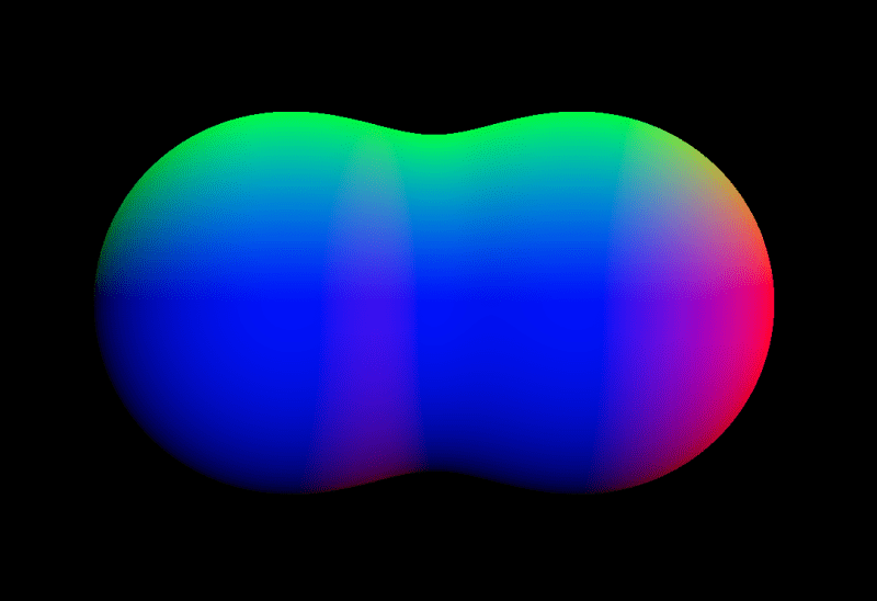
After we render the scene, you’ll discover that the floor of the sphere is shaded in pink, inexperienced, and blue primarily based on the orientation of the conventional vectors. It is because we’re mapping the 𝑥, 𝑦, and 𝑧 elements of the conventional vector to the RGB coloration channels respectively.

It is a frequent and intuitive method to debug regular vectors visually, serving to us guarantee they’re computed appropriately.

When combining two spheres with the usual min() perform, a tough edge types the place the shapes intersect, leading to an unnatural boundary.
To keep away from this, we will use a mixing perform referred to as smoothMin, which softens the transition by merging the space values easily.

// added
float smoothMin(float d1, float d2, float ok) {
    float h = exp(-k * d1) + exp(-k * d2);
    return -log(h) / ok;
}

float map(vec3 p) {
    float radius = 0.5;
    float ok = 7.; // added: smoothing issue for metaball impact
    float d = 1e5;

    float sphere0 = sdSphere(translate(p, vec3(.4, 0.0, 0.0)), radius);
    float sphere1 = sdSphere(translate(p, vec3(-.4, 0.0, 0.0)), radius);
    d = smoothMin(d, sphere0, ok); // modified: mix with smoothing
    d = smoothMin(d, sphere1, ok); // modified

    return d;
}

This perform creates a clean, steady connection between shapes—producing a metaball-like impact the place the types seem to merge organically.

The parameter ok controls the smoothness of the mix. The next ok worth leads to a sharper transition (nearer to min()), whereas a decrease ok produces smoother, extra gradual merging.

For extra particulars, please discuss with the next two articles:

4. Including Noise for a Droplet-like Look

Up to now, we’ve lined the way to calculate normals and the way to easily mix objects.

Subsequent, let’s tune the floor look to make issues really feel extra reasonable.

On this demo, we’re aiming to create droplet-like metaballs. So how can we obtain that sort of look? The important thing concept right here is to use noise to distort the floor.

Let’s soar proper into the code:

// output.frag

uniform float uTime;

// ...

float rnd3D(vec3 p) {
    return fract(sin(dot(p, vec3(12.9898, 78.233, 37.719))) * 43758.5453123);
}

float noise3D(vec3 p) {
    vec3 i = flooring(p);
    vec3 f = fract(p);

    float a000 = rnd3D(i); // (0,0,0)
    float a100 = rnd3D(i + vec3(1.0, 0.0, 0.0)); // (1,0,0)
    float a010 = rnd3D(i + vec3(0.0, 1.0, 0.0)); // (0,1,0)
    float a110 = rnd3D(i + vec3(1.0, 1.0, 0.0)); // (1,1,0)
    float a001 = rnd3D(i + vec3(0.0, 0.0, 1.0)); // (0,0,1)
    float a101 = rnd3D(i + vec3(1.0, 0.0, 1.0)); // (1,0,1)
    float a011 = rnd3D(i + vec3(0.0, 1.0, 1.0)); // (0,1,1)
    float a111 = rnd3D(i + vec3(1.0, 1.0, 1.0)); // (1,1,1)

    vec3 u = f * f * (3.0 - 2.0 * f);
    // vec3 u = f*f*f*(f*(f*6.0-15.0)+10.0);

    float k0 = a000;
    float k1 = a100 - a000;
    float k2 = a010 - a000;
    float k3 = a001 - a000;
    float k4 = a000 - a100 - a010 + a110;
    float k5 = a000 - a010 - a001 + a011;
    float k6 = a000 - a100 - a001 + a101;
    float k7 = -a000 + a100 + a010 - a110 + a001 - a101 - a011 + a111;

    return k0 + k1 * u.x + k2 * u.y + k3 *u.z + k4 * u.x * u.y + k5 * u.y * u.z + k6 * u.z * u.x + k7 * u.x * u.y * u.z;
}

vec3 dropletColor(vec3 regular, vec3 rayDir) {
    vec3 reflectDir = mirror(rayDir, regular);

    float noisePosTime = noise3D(reflectDir * 2.0 + uTime);
    float noiseNegTime = noise3D(reflectDir * 2.0 - uTime);

    vec3 _color0 = vec3(0.1765, 0.1255, 0.2275) * noisePosTime;
    vec3 _color1 = vec3(0.4118, 0.4118, 0.4157) * noiseNegTime;

    float depth = 2.3;
    vec3 coloration = (_color0 + _color1) * depth;

    return coloration;
}

// ...

void predominant() {
	// ...

	if ( dist < EPS ) {
		vec3 regular = generateNormal(ray);
		coloration = dropletColor(regular, rayDirection);
	}
	
	 gl_FragColor = vec4(coloration, 1.0);
}

To create the droplet-like texture, we’re utilizing worth noise. In the event you’re unfamiliar with these noise strategies, the next articles present useful explanations:

3D worth noise is generated by interpolating random values positioned on the eight vertices of a dice. The method includes three levels of linear interpolation:

Backside face interpolation: First, we interpolate between the 4 nook values on the underside face of the dice
Prime face interpolation: Equally, we interpolate between the 4 nook values on the highest face
Closing z-axis interpolation: Lastly, we interpolate between the outcomes from the underside and prime faces alongside the z-axis

This triple interpolation course of is named trilinear interpolation.

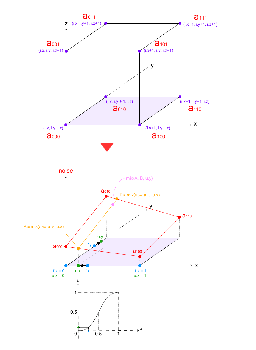
The next code demonstrates the trilinear interpolation course of for 3D worth noise:

float n = combine(
	combine( combine( a000, a100, u.x ), combine( a010, a110, u.x ), u.y ),
	combine( combine( a001, a101, u.x ), combine( a011, a111, u.x ), u.y ),
	u.z
);

The nested combine() features above could be transformed into an express polynomial kind for higher efficiency:

float k0 = a000;
float k1 = a100 - a000;
float k2 = a010 - a000;
float k3 = a001 - a000;
float k4 = a000 - a100 - a010 + a110;
float k5 = a000 - a010 - a001 + a011;
float k6 = a000 - a100 - a001 + a101;
float k7 = -a000 + a100 + a010 - a110 + a001 - a101 - a011 + a111;

float n = k0 + k1 * u.x + k2 * u.y + k3 *u.z + k4 * u.x * u.y + k5 * u.y * u.z + k6 * u.z * u.x + k7 * u.x * u.y * u.z;

By sampling this noise utilizing the reflection vector as coordinates, we will create a sensible water droplet-like texture. Notice that we’re utilizing the floor regular obtained earlier to compute this reflection vector. So as to add time-based variation, we generate noise at positions offset by uTime:

vec3 reflectDir = mirror(rayDir, regular);

float noisePosTime = noise3D(reflectDir * 2.0 + uTime);
float noiseNegTime = noise3D(reflectDir * 2.0 - uTime);

Lastly, we mix two noise-influenced colours and scale the end result:

vec3 _color0 = vec3(0.1765, 0.1255, 0.2275) * noisePosTime;
vec3 _color1 = vec3(0.4118, 0.4118, 0.4157) * noiseNegTime;

float depth = 2.3;
vec3 coloration = (_color0 + _color1) * depth;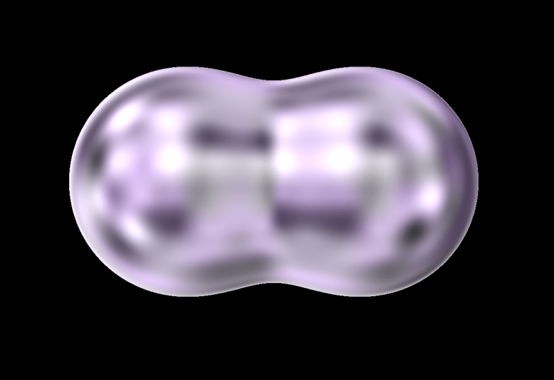

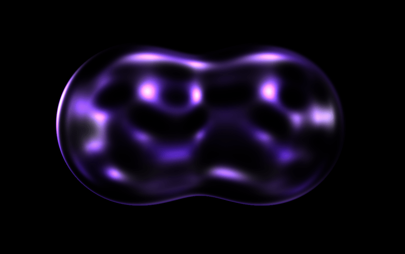
It’s beginning to look fairly like a water droplet! Nevertheless, it nonetheless seems a bit murky.
To enhance this, let’s add the next post-processing step:

// output.frag

if ( dist < EPS ) {
	vec3 regular = generateNormal(ray);
	coloration = dropletColor(regular, rayDirection);
}

vec3 finalColor = pow(coloration, vec3(7.0)); // added

gl_FragColor = vec4(finalColor, 1.0); // modified

Utilizing pow(), darker areas are suppressed, permitting the highlights to pop and making a extra glass-like, translucent floor.

5. Simulating Stretchy Droplets with Mouse Motion

Lastly, let’s make the droplet stretch and comply with the mouse motion, giving it a smooth and elastic really feel.

We’ll obtain this by inserting a number of spheres alongside the mouse path.

// Output.ts

constructor() {
	// ...
	this.trailLength = 15;
	this.pointerTrail = Array.from({ size: this.trailLength }, () => new THREE.Vector2(0, 0));
	
	this.uniforms = {
	    uTime: { worth: Widespread.time },
	    uResolution: {
	        worth: new THREE.Vector2(Widespread.width, Widespread.top),
	    },
	    uPointerTrail: { worth: this.pointerTrail },
	};
}

// ...

/**
 * # rAF replace
 */
replace() {
  this.updatePointerTrail();
  this.render();
}

/**
 * # Replace the pointer path
 */
updatePointerTrail() {
  for (let i = this.trailLength - 1; i > 0; i--) {
     this.pointerTrail[i].copy(this.pointerTrail[i - 1]);
  }
  this.pointerTrail[0].copy(Pointer.coords);
}

// output.frag

const int TRAIL_LENGTH = 15; // added
uniform vec2 uPointerTrail[TRAIL_LENGTH]; // added

// ...

// modified
float map(vec3 p) {
    float baseRadius = 8e-3;
    float radius = baseRadius * float(TRAIL_LENGTH);
    float ok = 7.;
    float d = 1e5;

    for (int i = 0; i < TRAIL_LENGTH; i++) {
        float fi = float(i);
        vec2 pointerTrail = uPointerTrail[i] * uResolution / min(uResolution.x, uResolution.y);

        float sphere = sdSphere(
                translate(p, vec3(pointerTrail, .0)),
                radius - baseRadius * fi
            );

        d = smoothMin(d, sphere, ok);
    }

    float sphere = sdSphere(translate(p, vec3(1.0, -0.25, 0.0)), 0.55);
    d = smoothMin(d, sphere, ok);

    return d;
}

Conclusion

On this tutorial, we explored the way to create a dynamic, droplet-like impact utilizing ray marching and shading strategies. Right here’s what we lined: