On this article, you’ll learn the way a vector database works beneath the hood by constructing one from scratch in ten incremental steps utilizing Python and NumPy.
Matters we are going to cowl embrace:
- How paperwork are encoded into fixed-size vectors and searched by that means reasonably than by key phrase.
- The right way to add metadata filtering, enter validation, and persistence to a minimal vector database.
- How brute-force cosine similarity scales with corpus dimension, and when to think about approximate indexing.
Introducing Vector Databases
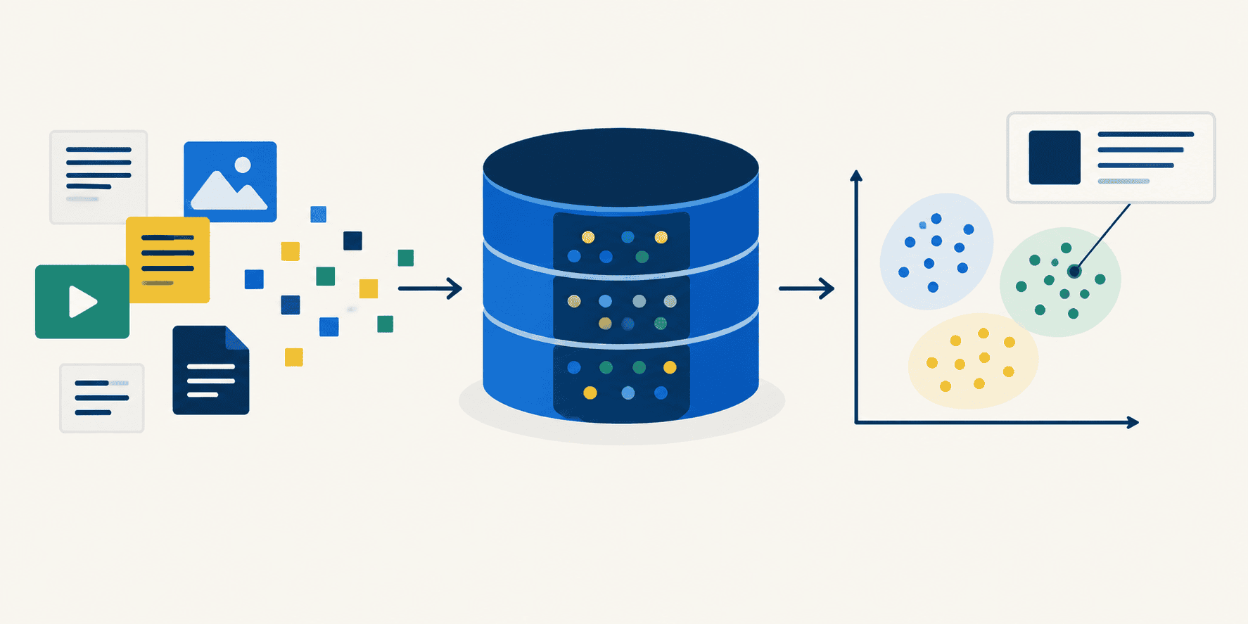
A vector database solutions questions by that means reasonably than by key phrase. It operates by turning each doc right into a vector of numbers after which discovering the numbers that time in an analogous route to your question (which has additionally been become a vector of numbers). This tutorial will reveal find out how to construct a working vector database of your very personal, by way of ten steps that every reveal one atomic concept. To comply with alongside, create an empty script and identify it one thing intelligent like tutorial.py. Append every step’s code to the script as you go and re-run it after you make sense of the commentary. The ensuing output ought to make sense at that time. Nothing right here wants a GPU or an API key; one small mannequin downloads on the primary run, and all the pieces after that’s plain NumPy.
Step 1: Setup
You want three recordsdata from this repository in your working listing: vector_db.py is the precise database which, sure, is already constructed for you… however the actual magic is the understanding of the code and the interplay with it utilizing the code herein. The excellent news is, when you undergo this tutorial and perceive the code, recreating the vector database by yourself is almost trivial. corpus.py accommodates 25 simulated pattern paperwork and their matter tags. take a look at.py is the take a look at suite, solely right here to make you are feeling secure and safe that the vector database works correctly as applied, which you’ll confirm by operating at any level with python take a look at.py.
Set up the 2 dependencies:
|
pip set up numpy sentence–transformers |
Now begin your tutorial.py file with the imports and two small show helpers. present() prints a listing of search outcomes as rating, matter, doc (relied upon later). header() simply labels every part so the rising script’s output stays readable.
|
1 2 3 4 5 6 7 8 9 10 11 12 13 14 15 16 17 18 19 20 |
import time from pathlib import Path
import numpy as np
from corpus import DOCS, META from vector_db import VectorDB
WIDTH = 64
def header(title): print(f“n{title}n{‘─’ * len(title)}”)
def present(outcomes): if not outcomes: print(” (no matches)”) for hit in outcomes: textual content = hit.textual content if len(hit.textual content) <= WIDTH else hit.textual content[: WIDTH – 1] + “…” print(f” {hit.rating:+.3f} [{hit.meta[‘topic’]:<7}] {textual content}”) print() |
Working the script now produces no output. That is what we would like; nothing has been known as but.
Step 2: Constructing the Index
Making a VectorDB masses the embedding mannequin, and add() encodes each doc right into a vector and shops it.
|
header(“2. Constructing the index”)
t0 = time.perf_counter() db = VectorDB() load_seconds = time.perf_counter() – t0
t0 = time.perf_counter() db.add(DOCS, META) encode_seconds = time.perf_counter() – t0
print(f” {db!r}”) print(f” mannequin load: {load_seconds:5.2f}s”) print(f” encoding: {encode_seconds:5.2f}s for {len(db)} paperwork “ f“({encode_seconds / len(db) * 1000:.0f} ms every)”) print(f” index dimension: {db.vectors.nbytes / 1024:5.1f} KiB “ f“{db.vectors.form} of {db.vectors.dtype}”) |
Output:
|
2. Constructing the index ───────────────────── VectorDB(25 docs, dim=384, mannequin=‘sentence-transformers/all-MiniLM-L6-v2’) mannequin load: 1.64s encoding: 0.14s for 25 paperwork (6 ms every) index dimension: 37.5 KiB (25, 384) of float32 |
Word that the index dimension doesn’t depend upon how lengthy the paperwork are. Each doc, whether or not a six-word sentence or a six-page essay, turns into the identical 384 numbers at 4 bytes every: 1,536 bytes, flat. That’s mounted, and is what makes a vector index predictable to dimension and low-cost to scan.
Step 3: A First Search
|
header(“3. A primary search”)
question = “what retains a cell equipped with power?” print(f‘ question: “{question}”n’) present(db.search(question, okay=3)) |
Output:
|
3. A first search ───────────────── question: “what retains a cell equipped with power?”
+0.589 [bio ] The mitochondria is the powerhouse of the cell. +0.440 [bio ] Throughout cardio respiration, mitochondria produce ATP by way of th... +0.329 [comics ] Thor‘s mitochondria–wealthy muscle fibres make him a organic po... |
The highest hit shares precisely one phrase with the question (“cell”) and the runner-up shares none in any respect. A key phrase index would have ranked these very in a different way, if it discovered them in any respect.
Step 4: Looking out With out Sharing a Single Phrase
|
header(“4. Looking out with out sharing a single phrase”)
for question in (“why does my loaf style bitter”, “superheroes”): print(f‘ question: “{question}”n’) present(db.search(question, okay=3)) |
Output:
|
4. Looking out with out sharing a single phrase ────────────────────────────────────────── question: “why does my loaf style bitter”
+0.630 [food ] The tangy flavour of sourdough bread comes from acetic and lact... +0.497 [food ] Sourdough fermentation depends on wild yeast and lactic acid bac... +0.386 [food ] The Maillard response between amino acids and decreasing sugars i...
question: “superheroes”
+0.369 [comics ] Tony Stark‘s alter ego Iron Man wields a powered exoskeleton ar... +0.357 [comics ] Peter Parker gained tremendous–power, wall–crawling, and a precog... +0.353 [comics ] Bruce Banner involuntarily transforms into the Hulk when his advert... |
That is the entire level of the train. Neither question shares any phrase with the paperwork it retrieves; no situations of “loaf”, “bitter”, nor “superhero” seem anyplace within the corpus. The match is on that means.
Step 5: Studying The Scores
|
header(“5. Studying the scores”)
question = “one of the simplest ways to vary a tyre” print(f‘ question: “{question}”n’) present(db.search(question, okay=3)) |
Output:
|
5. Studying the scores ───────────────────── question: “one of the simplest ways to vary a tyre”
+0.111 [ml ] Transformers changed recurrent networks for most sequence duties. +0.096 [comics ] Like Peter Parker‘s cells continually regenerating thanks to his... +0.068 [ml ] The self–consideration mechanism in transformers permits every token ... |
A vector search at all times returns okay outcomes, even when the corpus holds nothing related; it merely ranks what it has. The rating is the one sign of whether or not a solution is any good: examine the +0.111 right here towards the +0.630 in step 4. In manufacturing you’d set a ground and return nothing under it.
Step 6: Narrowing Outcomes with Metadata
Each doc was added with a {"matter": ...} dict. The the place argument retains solely the paperwork whose metadata matches on each key given.
|
header(“6. Narrowing outcomes with metadata”)
question = “what retains a cell equipped with power?” print(f‘ question: “{question}” (no filter)n’) present(db.search(question, okay=4))
print(f‘ question: “{question}” the place={{“matter”: “bio”}}n’) present(db.search(question, okay=4, the place={“matter”: “bio”})) |
Output:
|
6. Narrowing outcomes with metadata ────────────────────────────────── question: “what retains a cell equipped with power?” (no filter)
+0.589 [bio ] The mitochondria is the powerhouse of the cell. +0.440 [bio ] Throughout cardio respiration, mitochondria produce ATP by way of th... +0.329 [comics ] Thor‘s mitochondria–wealthy muscle fibres make him a organic po... +0.308 [bio ] Mitochondria comprise their personal DNA, a remnant of their historical ...
question: “what retains a cell equipped with power?” the place={“matter”: “bio”}
+0.589 [bio ] The mitochondria is the powerhouse of the cell. +0.440 [bio ] Throughout cardio respiration, mitochondria produce ATP by way of th... +0.308 [bio ] Mitochondria comprise their personal DNA, a remnant of their historical ... +0.191 [bio ] Mitochondrial dysfunction has been linked to neurodegenerative ... |
The corpus accommodates a deliberate lure: a comics doc about Thor’s “mitochondria-rich muscle fibres” that may be a genuinely good vector match for a biology query. Filtering is the way you rule it the match — similarity alone can’t, as a result of by that means it actually is analogous.
Step 7: A Filter Narrower Than okay
|
header(“7. A filter narrower than okay”)
print(‘ question: “bread” the place={“matter”: “music”}, okay=5n’) outcomes = db.search(“bread”, okay=5, the place={“matter”: “music”}) present(outcomes) print(f” requested for five, bought {len(outcomes)}n”)
print(‘ question: “bread” the place={“matter”: “astrology”}n’) present(db.search(“bread”, okay=5, the place={“matter”: “astrology”})) |
Output:
|
7. A filter narrower than okay ─────────────────────────── question: “bread” the place={“matter”: “music”}, okay=5 +0.082 [music ] In classical music, a fugue is a contrapuntal composition in wh... requested for 5, bought 1
question: “bread” the place={“matter”: “astrology”} (no matches) |
Just one doc is tagged music, so asking for five returns 1. Outcomes are filtered earlier than they’re ranked, that means {that a} non-matching doc can by no means be padded into the listing simply to succeed in okay.
Step 8: Guard Rails
|
header(“8. Guard rails”)
for label, texts, metadata in [ (“a single string instead of a list”, “one document”, None), (“metadata that does not line up”, [“a”, “b”, “c”], [{“topic”: “x”}]), ]: strive: db.add(texts, metadata) besides (TypeError, ValueError) as err: print(f” {label}:n {sort(err).__name__}: {err}n”) |
Output:
|
8. Guard rails ────────────── a single string as a substitute of a listing: TypeError: add() takes a listing of strings, not a single string
metadata that does not line up: ValueError: bought 3 texts however 1 metadata entries; they should line up one–to–one |
add() retains paperwork, metadata and vectors in lockstep. Each of the above errors are straightforward to make and would silently corrupt an index if not caught. A naked string is iterable, so docs.prolong("hello") would append “h” and “i” as two separate paperwork, and the mannequin returned a single vector.
Step 9: Saving and Loading
|
header(“9. Saving and loading”)
db.save(“index”) for path in sorted(Path(“index”).iterdir()): print(f” {path} {path.stat().st_size / 1024:6.1f} KiB”)
reopened = VectorDB() reopened.load(“index”) print(f“n reopened: {reopened!r}”) print(f” vectors equivalent: {np.array_equal(db.vectors, reopened.vectors)}”) print(f” similar prime hit: {reopened.search(‘superheroes’, okay=1)[0].textual content[:44]}…”) |
Output:
|
9. Saving and loading ───────────────────── index/retailer.json 3.0 KiB index/vectors.npy 37.6 KiB
reopened: VectorDB(25 docs, dim=384, mannequin=‘sentence-transformers/all-MiniLM-L6-v2’) vectors equivalent: True similar prime hit: Tony Stark‘s alter ego Iron Man wields a pow... |
The vectors go to .npy as a result of it’s compact and masses with out parsing. The textual content and metadata go to .json so you’ll be able to open the file and browse it. load() refuses an index constructed by a special mannequin. That is necessary as a result of embeddings solely imply one thing relative to the mannequin that produced them; mixing them wouldn’t be slightly bit “off,” it could be assured nonsense.
Step 10: How This Scales
Twenty-five paperwork are too few to measure, so this step additionally instances an artificial corpus of random vectors. They rating meaningless outcomes, however the computational price matches an actual world state of affairs.
|
1 2 3 4 5 6 7 8 9 10 11 12 13 14 15 16 17 18 19 20 21 22 23 24 25 26 27 28 29 30 31 |
header(“10. How this scales”)
runs = 50 t0 = time.perf_counter() for _ in vary(runs): db.search(“reminiscence security and not using a rubbish collector”, okay=5) print(f” {(time.perf_counter() – t0) / runs * 1000:.1f} ms per question “ f“over {len(db)} documentsn”)
rng = np.random.default_rng(0) huge = rng.random((100_000, db.dim), dtype=np.float32) huge /= np.linalg.norm(huge, axis=1, keepdims=True) query_vector = huge[0]
def milliseconds(work, repeats=20): work() t0 = time.perf_counter() for _ in vary(repeats): work() return (time.perf_counter() – t0) / repeats * 1000
print(f” {‘paperwork’:>12} {‘reminiscence’:>9} {‘scan’:>9} {‘rank’:>9}”) for n in (1_000, 10_000, 100_000): rows = huge[:n] scores = rows @ query_vector scan_ms = milliseconds(lambda: rows @ query_vector) rank_ms = milliseconds(lambda: np.argsort(scores)[::–1][:5]) print(f” {n:>12,} {rows.nbytes / 1024**2:>7.1f} MB “ f“{scan_ms:>6.2f} ms {rank_ms:>6.2f} ms”) |
Output:
|
10. How this scales ────────────────── 14.9 ms per question over 25 paperwork
paperwork reminiscence scan rank 1,000 1.5 MB 0.01 ms 0.04 ms 10,000 14.6 MB 0.36 ms 0.55 ms 100,000 146.5 MB 3.73 ms 8.90 ms |
At 25 paperwork, embedding the question is actually all the computation, because the search itself is simply too quick to measure. Word that milliseconds() discards one warm-up run; the primary name to a NumPy matrix routine spins up its inner thread pool, which may take extra time than the precise work itself, with a results of making a small corpus look slower than a big one.
Two issues are value declaring within the outcomes desk above:
- Each columns develop linearly; nothing right here is intelligent, it merely touches each row.
- Previous ~100,000 rows the kind begins to outgrow the scan. At 1,000,000 paperwork the scan takes about 25 ms and the total type about 90 ms. That’s the level the place it pays to cease sorting all the pieces (
np.argpartitionfinds the highestokayin about 10 ms). Not far past this you can see the purpose the place you attain for an actual approximate index (HNSW, IVF) and commerce slightly accuracy for pace.
Wrapping Up
Each step right here rests on a single concept: scale every embedding to size 1, and a plain dot product turns into cosine similarity. Rating a whole corpus is then one matrix multiply. Every little thing else you added alongside the best way — from metadata filters, saving and loading, the guard rails on add() — is bookkeeping that retains paperwork, metadata and vectors in lockstep, in order that the multiplication stays significant.
The massive takeaway — past the simplicity and magnificence behind the implementation of a vector database’s core performance — is that the design doesn’t change between 25 paperwork and 25 million; solely the index construction beneath it does. That is, not surprisingly, exactly what the managed vector databases are promoting.
For extra info on vector databases from totally different factors of view, take a look at these Machine Studying Mastery assets: